As foundation models scale to billions of parameters, they become more prone to training instability. During pretraining or large fine-tuning runs, it is common to see loss spikes, silent non-convergence, or sudden divergence to NaN values. These failures are often connected to vanishing or exploding gradients.
In this post, we look at why gradients explode or vanish, why foundation models are sensitive to these issues, how to track gradients across layers, and which stabilization techniques are most useful.
What gradient issues occur during training?
Foundation models are usually trained with adaptive gradient-based optimizers such as Adam or AdamW. At a high level, parameters are updated by subtracting a scaled gradient of the loss:
theta = theta - learning_rate * gradient(loss, theta)During the forward pass, the model computes predictions and loss. During the backward pass, gradients are propagated through the model using the chain rule. In deep architectures, repeated multiplication through many layers can shrink gradients toward zero or make them grow uncontrollably.
Vanishing gradients
Vanishing gradients occur when gradients become extremely small as they move backward through the network. Earlier layers then receive almost no useful update. Training becomes slow, unstable, or effectively frozen.
This can happen when activation derivatives are small, when many units are inactive, or when weight matrices have norms below one across many layers. With ReLU, for example, inactive neurons have zero derivative, so gradient flow stops for those paths. In very deep networks, even small shrinkage at each layer can compound into a near-zero signal.
Exploding gradients
Exploding gradients are the opposite failure mode. Gradients grow exponentially during backpropagation, causing large parameter updates. The model may oscillate, diverge, or produce NaN loss values.
This often happens when the product of weight norms and activation derivatives is repeatedly greater than one. In large-scale models, the issue can appear as sudden loss spikes, instability in specific blocks, or training collapse during early optimization.
Why track gradients layer by layer?
Layer-wise gradient monitoring helps with three stages of debugging.
- Discovery: confirm whether gradients are becoming too small, too large, or NaN during training.
- Root-cause analysis: identify which layer, block, or parameter group first becomes unstable.
- Validation: check whether a mitigation strategy, such as clipping or learning-rate changes, actually improves training.
Gradient-norm tracking in PyTorch
Gradient norm tracking calculates the norm of gradients for selected model parameters during backpropagation. The L2 norm is commonly used because it gives a smooth measure of gradient magnitude and makes extreme values easy to spot.
The runnable notebook tracks a BERT-style sequence classification model in PyTorch and plots the metrics directly in Colab. For large models, you should usually log selected layers or aggregate norms at the block level rather than logging every parameter every step.
Step 1: Create a local metric history
history = []

def log_metrics(metrics, step):
    history.append({"step": step, **metrics})
This keeps the demo self-contained. In a production run, the same metric dictionary can be sent to a real experiment tracker only after the project exists and the link has been verified.
Step 2: Define a gradient logging function
import torch

def log_gradient_norms(model, step, log_every_n_steps=1):
    """Record L2 gradient norms for model parameters."""
    if step % log_every_n_steps != 0:
        return

    metrics = {}
    with torch.no_grad():
        for name, param in model.named_parameters():
            if param.grad is not None:
                metrics[f"gradients/{name}"] = param.grad.norm().item()

    log_metrics(metrics, step=step)
Computing L2 norms is inexpensive, but logging every parameter in a foundation model can become noisy and costly. In practice, monitor the most informative components: embeddings, attention layers, MLP blocks, output heads, or aggregated block-level norms. Reducing logging frequency, for example logging every 10 or 100 steps, also helps.
Step 3: Train and log loss
import torch.optim as optim

optimizer = optim.Adam(model.parameters(), lr=1e-1)
model.train()

global_step = 0
for epoch in range(10):
    for batch in train_dataloader:
        inputs = {
            key: value.to("cuda")
            for key, value in batch.items()
            if key in tokenizer.model_input_names
        }
        labels = batch["labels"].to("cuda")

        optimizer.zero_grad()
        outputs = model(**inputs, labels=labels)
        loss = outputs.loss
        loss.backward()

        log_gradient_norms(model, global_step, log_every_n_steps=10)
        optimizer.step()

        log_metrics({"loss": loss.item()}, step=global_step)
        global_step += 1
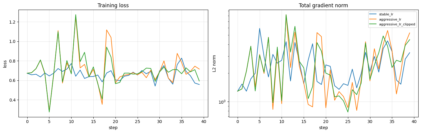
If the learning rate is too high, loss and gradient norms may quickly diverge to NaN. If the learning rate is too low, the loss may stay high while gradients in some layers shrink. The point of tracking gradients is to see where that behavior begins, not just that the final loss looks bad.
Diagnosing training issues
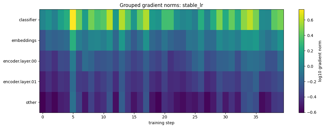
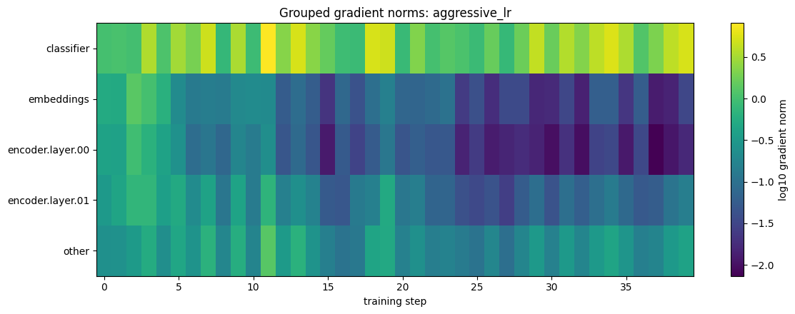
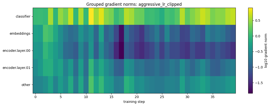
Once gradient tracking is in place, compare loss curves with layer-wise gradient norms. If loss diverges and gradient norms explode in later layers first, the learning rate may be too aggressive or clipping may be needed. If earlier blocks show near-zero gradients while the output layer still changes, you may be seeing vanishing gradients or inactive layers.
In one typical BERT-style debugging setup, a very large learning rate can cause both loss and gradient norms to become NaN within a few steps. Reducing the learning rate may prevent immediate divergence, but the model can still fail to converge if gradients in key layers do not evolve. Lowering the learning rate further, adding warmup, or adjusting initialization can produce smoother loss and more meaningful gradient flow.
Techniques for gradient stabilization
- Gradient clipping: caps gradient magnitude during backpropagation and prevents unusually large updates.
- Layer normalization: stabilizes activation scales across features and is a standard component in transformer-based foundation models.
- Weight initialization: Xavier, He, truncated normal, and architecture-specific initialization schemes help preserve signal scale across layers.
- Activation functions: GELU, Swish, and LeakyReLU can avoid some failure modes associated with plain ReLU in very deep networks.
- Learning-rate schedules: warmup and decay reduce early training shocks and help avoid unstable updates.
Wrapping up
Gradient issues can quietly prevent large models from learning. Tracking gradient norms across layers makes the training process more observable: you can see where gradients vanish, where they explode, and whether a fix actually improves the run.
The Colab notebook keeps the demo local, but the same metrics can be sent to an experiment tracker once a real project exists. The more expensive the training run, the more valuable this kind of visibility becomes.